Phase and Group Velocity in wave propagation

A harmonic wave is a disturbance that varies in space and time according to a sinusoidal function—a periodic trigonometric function of the form
(1) y(x, t) = A cos(kx – ωt + φ)
that describes a smooth, regular oscillation between a maximum and a minimum value. Phase velocity and group velocity represent two distinct metrics for measuring the propagation of such a wave, depending on whether the focus is on an individual oscillation or on the overall envelope structure of the signal.

When considering an ideal monochromatic wave, the phase velocity (vf = ω / k) quantifies the rate at which a point of constant phase moves through space—that is, the displacement speed of a single crest or trough of the sinusoid. However, physical waves capable of transmitting information are never purely monochromatic; they consist of a superposition of spectral components across a range of frequencies (1), forming what is known as a wave packet. The group velocity (vg = dω / dk) precisely measures the propagation speed of the overall envelope of this wave packet.

The core distinction between these two quantities lies in their underlying physical significance. While the phase velocity describes strictly the motion of the oscillatory state and can, in specialized media such as certain plasmas or metamaterials, exceed the speed of light in vacuum c, the group velocity represents the effective speed at which physical energy and signal information travel.
In non-dispersive media—where all spectral components propagate at the same speed—the two values are identical (vf = vg). Conversely, in dispersive media, the frequency dependence of the medium’s properties causes a dispersion relation where the two velocities diverge, typically resulting in a group velocity that is lower than the phase velocity (vg < vf).


In the image the red dot propagates with phase velocity while the green dots propagate with group velocity, source Wikipedia.

Wave group

please, rate this post

Mathematical and historical foundations of Extended Theories of Gravity (ETG)

A short paper, in english, on a fascinating development of General Relativity.

Abstract
Extended Theories of Gravity (ETG) represent a prominent framework in modern theoretical physics and cosmology, aimed at modifying or extending Albert Einstein’s General Relativity to address open phenomenological questions at both ultraviolet (early universe) and infrared (galactic and cosmological) scales.

pdf Brussi 2026 Mathematical and historical foundations of ETG (305 KB)

ETG

please, rate this post

Galactic Energy Profiles II

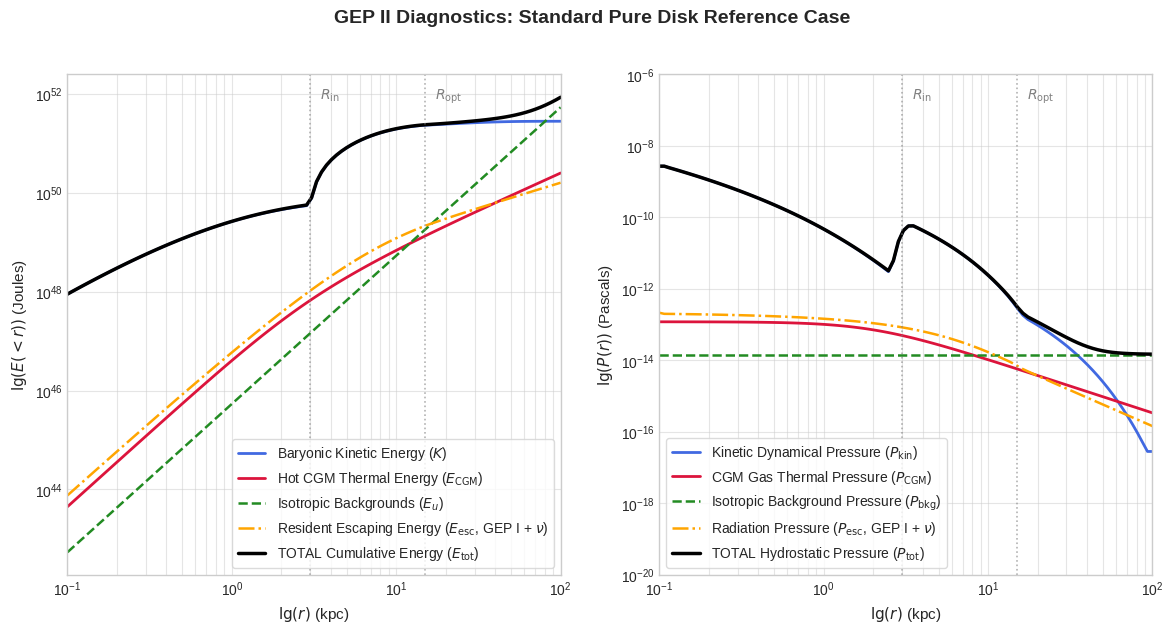
Galactic Energy Profiles: GEP II. In-System and Background Energy Densities

Update: I decided to publish this work, part of the GEP series, on Zenodo without peer review and to use it as a basic tool for building a subsequent dataset (GEP III). Note: This work is version 2.0 of the previous NAGE II work, which has been superseded.


Abstract
Standard galactic energy inventories typically focus on virialized components, namely kinetic and gravitational potential energy derived from baryonic mass distributions, together with energy inferred from bolometric luminosities. In the first paper of the Galactic Energy Profiles (GEP) series, we introduced a reproducible geometric framework for the radiant and relativistic fluxes of galactic origin, accounting for their finite escape time across the Halo. In this second work, we extend the framework toward a volumetric energy inventory, where bolometric luminosity is complemented by energy densities persistently present within the galactic volume. We consider the thermal and kinetic energy of baryonic matter—including bulk motions, turbulence, and rotational degrees of freedom from large-scale dynamics down to the intrinsic angular momentum of bound systems—together with cosmic rays confined by magnetic fields and extragalactic backgrounds (photons, neutrinos, and diffuse fields) permeating the Halo. This approach distinguishes between flux-based contributions and volume-based reservoirs, providing a complementary description of the total galactic energy budget. Crucially, by resolving these volumetric reservoirs into local radial profiles, we characterize the multi-component pressure support (including thermal, magnetic, cosmic ray, and radiant pressures) available to sustain the circumgalactic medium (CGM) in hydrostatic equilibrium. Although these components vary with morphology and evolutionary state, this study is purely theoretical and simplifies the extreme variability of galactic systems to derive reference estimates and ‘standard cases’. The resulting parametrized framework, supported by publicly available Python scripts, is intended as a further methodological baseline for the sample-wide application planned in later work.

Keywords
galactic energy inventory; galactic energy density; galactic Halo energy; energy distribution based on galactic morphology


Here is the Zenodo version of the paper (1.1 MB):

pdf Brussi 2026_GEP II


GEP_II

please, rate this post

Galactic Energy Profiles I

Galactic Energy Profiles: GEP I. Radiant and Relativistic Fluxes

Update: I decided to publish this work, part of the GEP series, on Zenodo without peer review and to use it as a basic tool for building a subsequent dataset (GEP III). Note: This work is version 2.0 of the previous NAGE I work, which has been superseded.


Abstract
Standard galactic energy inventories typically focus on the virialized components of the system, namely the kinetic and gravitational potential energy, derived from baryonic mass distributions and stellar luminosity. This paper, the first in the Galactic Energy Profiles series, introduces a reproducible geometric framework for accounting radiant and relativistic fluxes as a standing energy reservoir. By considering the photon and neutrino escape time τ across the galactic Halo, we quantify the energy density of radiation currently in transit as a component of the total galactic budget, complementary to the standard flux-based description. The resulting closed-form expressions, together with the accompanying open-source Python implementation, are intended as a calibrated methodological baseline for the subsequent application of this framework to observed galactic samples.

Keywords
galactic energy inventory; energy residence time; galactic radiant fluxes; galactic Halo energy; galaxy morphology


Here is the Zenodo version of the paper (1.1 MB):

pdf Brussi 2026 GEP I


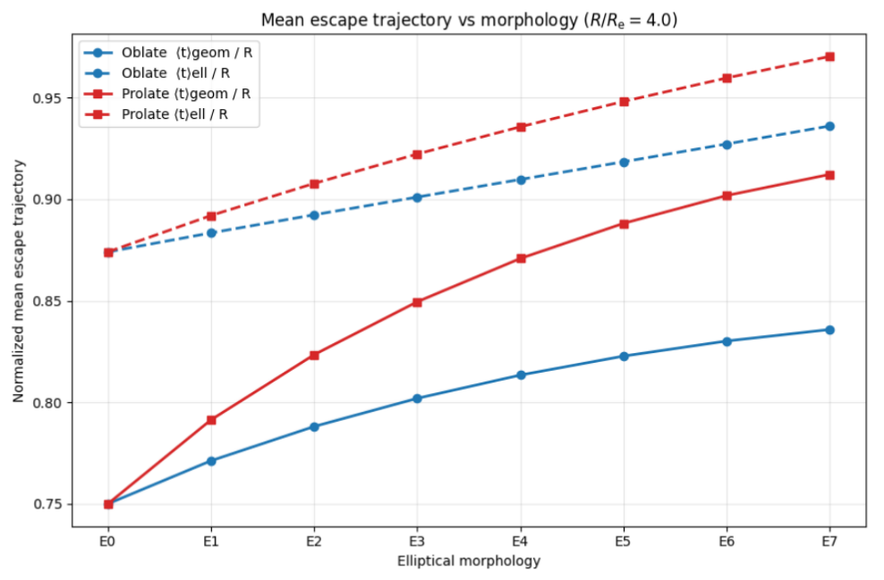
GEP I mean escape trajectory length

please, rate this post

Einstein’s formula for energy

The most famous physics formula in the world is probably that of Albert Einstein (1879-1955):
(1) E = mc²
that is, the energy of a body is equal to its mass times the speed of light squared.
Perhaps not many have truly understood it, but certainly almost no one (without university studies) knows the complete formula, which takes into account both moving bodies and the energy of massless particles.

For moving bodies, a multiplication factor must be considered:
(2) E = γ mc²
According to Einstein’s own special relativity (work from 1905), if we consider ‘particles’ moving in four-dimensional spacetime, the change in their momentum (p), is expressed by the relativistic formula of four-momentum. This is a four-vector* in which the time component is represented by energy and the space components by momentum. In particular, in the case of a moving body, its inertia increases, as in (2), according to a factor proportional to the velocity, called the Lorentz factor (after Hendrik Lorentz, 1853-1928):
γ = 1 / √ (1-v²/c²)
where v is the velocity of the body and c is the speed of light. As can be seen from the formula and from Figure 1 which traces its progression, γ increases as the velocity increases, but remains very close to 1 until the velocities are of the order of magnitude of that of light. For this reason, it is generally omitted, considering γ ≈ 1 . The asymptotic behavior of γ also highlights the difficulty of accelerating material bodies to speeds approaching that of light, whose inertia would have an equally asymptotic behavior.


Figura 1 (credits: youmath.it)
gamm


But the four-momentum also takes into account particles that have no mass, such as photons. From the intuition of Louis de Broglie (1892-1987), the wavelength of a photon is inversely proportional to its momentum:
λ = h / p
where h is Planck’s constant. Recalling that the photon’s energy can be expressed as:
E = hc / λ
it is easy to obtain the relation:
(3) E = pc

Einstein’s complete formula for the energy equation is therefore:
(4) E² = (pc)² + (mc²)²

It is easy to see how, in the case of a massless photon, (4) reduces to (3), the energy of the photon, and in the case of a non-moving particle, (4) reduces to (1), the energy of matter at rest. In the case of a moving body, both the energy due to the movement and the energy at rest must be taken into account, i.e. relation (2).


  • A four-vector is a four-dimensional vector defined in (relativistic) Minkowski (Hermann Minkowski 1864-1909) spacetime. It unifies a temporal quantity and the three corresponding spatial quantities (for example, time and space, or energy and momentum) into a single mathematical object.
    Its fundamental characteristic is that its magnitude (its length) remains unchanged for every observer, ensuring that the laws of physics remain the same even when observed from reference frames in relative motion to each other.
please, rate this post

The Stage of Reality – Why gravity is not a force and the speed of light is not a speed

Introduction
What we are about to explore is what I call ‘the stage of reality’, the place where we, and everything around us, move (a trivial side note: nothing is truly ‘at rest’ in our universe, as there is no absolute reference frame against which to measure motion). This stage is what we call spacetime, composed of the three familiar spatial dimensions plus time, which is simply an additional dimension. We cannot ‘visualize’ it unless we imagine removing one of the spatial dimensions, as seen in the famous Minkowski diagrams (see Figure, Hermann Minkowski, 1864-1909).
It was Albert Einstein (1879-1955), in his brilliant work in the early 1900s, who viewed the universe not as an empty space where time flows separately, but as a single four-dimensional context. These dimensions are inextricably linked by a metric governed by the laws of gravitation. In this scenario, time is not an external clock, but a real direction in which we move, just as we move North or South, to put it in geographic terms.

Gravity
Why is the force of gravity not a force? For centuries, thanks to Isaac Newton (1643-1727), we thought of gravity as a kind of ‘invisible hand’ that ‘pulls’ objects. But if we apply what Einstein called the equivalence principle (which he described as “the happiest thought of my life”), we discover a fundamental concept. He imagined being in an elevator in deep space, far from any gravitation, accelerating upwards (remember that acceleration is the variation of velocity). You would feel pressed to the floor exactly as you do on Earth. If you were to release Newton’s legendary apple, it would ‘fall’ toward the floor. Yet, there is no gravity ‘pulling’ it; there is only acceleration. Einstein realized that gravity is not a force acting in space; rather, the effect we observe and call ‘force’ is the consequence of the curvature of spacetime itself. In fact, the presence of mass —or rather, mass-energy, since they are the same thing except for a conversion factor (the famous E=mc² )— warps the fabric of spacetime like a weight on an elastic sheet. For example, the Earth, with its concentration of mass-energy, creates a geometric deformation: the apple doesn’t fall because a force pushes it, but because it is simply following the straightest possible line (called a geodesic) in a space that has become curved.
According to Newton’s laws of motion, a body with no forces acting upon it moves with uniform rectilinear motion (respecting the principle of inertia). According to Relativity, an apple falling in a gravitational field is, paradoxically, the only object experiencing no force at all (respecting the principle of inertia). To quote Einstein again: “Matter [mass-energy] tells spacetime how to curve, and spacetime tells matter how to move.”

Light
Now let’s consider light. We attribute a ‘speed’ to it (which we define as a change in position), but as physicist Leonard Susskind (1940-) explains, it is not a speed in the common sense of the term (like that of a car). Instead, it is a fundamental property of the geometry of spacetime —a simple ‘conversion factor’ between spatial and temporal coordinates.
In the four-dimensional universe in which we exist, space and time are different directions of the same thing, and  c  is the number that tells us how many meters are equivalent to one second. That is: time=space / c .
The value of the universal constant c is approximately 300,000 km per second, or just over a billion km per hour (approx. 1.08 billion km/h).
Susskind’s profound suggestion is that every object in the universe always and constantly moves at the exact same speed:
– When we are ‘still’ in space—for instance, sitting in our chairs—we are traveling at the speed of light along the axis of time
– If we start moving through space, we must ‘subtract’ speed from time to compensate for the spatial movement (as if paying a toll using the conversion factor, ). From this, the relativistic time dilation is derived (e.g., the twin paradox).
There are no variable speeds; there is only a distribution of the ‘total speed’ among different dimensions. Therefore, light isn’t ‘racing’: we could say that light spends its entire ‘allowance’ on space, leaving zero for time, based on the conversion factor c .
This constant —the speed of light— is the geometric limit of what can happen in the universe.

Conclusions
There is, therefore, no speed limit; there is only a global geometry in which we are all immersed. Gravity is the curvature of the road; the constant holds together the very fabric of the reality surrounding us. Physics does not describe ‘what happens’, but describes the geometric structure in which everything is already contained.
Understanding this means stopping looking at ‘things’ that move and starting to look at the shape of the stage on which they move.


A Minkowsky diagram (credits to medium.com)
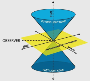

MInkowsky diagram

please, rate this post

The URD Framework – under development

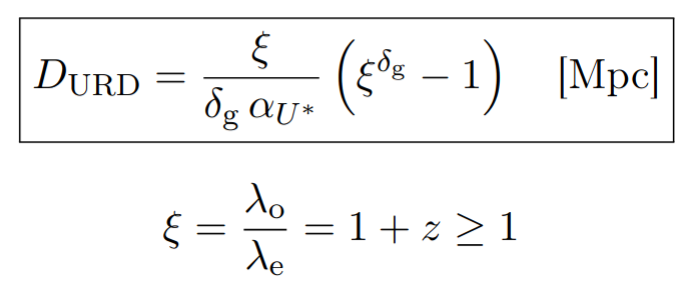
The URD Framework: Cosmological Distances from Redshift in a Non-Standard Context

While I am still developing the project —including through parallel studies on the Tolman test and the quality of indirect data obtained from recent galaxy surveys— I am making my work public as a preprint. I always hope that someone might be interested in my conjectures or perhaps even willing to collaborate with me to address the critical issues of the URD Framework.


Abstract
A phenomenological framework for determining cosmological distances is proposed, based on a non-expanding spacetime interpretation consistent with current observational datasets. The model introduces a redshift mechanism associated with cumulative photon energy attenuation along the line of sight, formulated in a way that is not equivalent to standard tired light scenarios. The approach is constructed to remain compatible with established relativistic principles whereas adopting boundary conditions distinct from the metric expansion paradigm. Distance estimation is achieved through the URD equation (U energy density, Redshift, Distance), which incorporates two phenomenological parameters that describe conformal geometric dissipation in extended gravity and an effective relativistic path-length correction. Within this formulation, the model addresses the primary shortcomings traditionally associated with energy dissipation effects, specifically reconciling time dilation in supernova light curves and the Tolman surface brightness relation. The model is calibrated using the Pantheon+ supernova sample by comparing and cross-validating distances inferred from the proposed redshift mapping with redshift-independent indicators, with additional comparison performed against baryon acoustic oscillations, radio galaxy samples, and high-energy quasars. Across these datasets, the framework reproduces observational constraints over a wide redshift range within a phenomenological, non-standard cosmological setting. The results indicate that alternative, non-expansion-based mappings between redshift and distance can be constructed that remain consistent within the observational range considered, suggesting a phenomenological alternative worth further study.
Keywords
cosmological distance ladder; redshift-distance relation; non-expanding spacetime; cosmic microwave background; extended gravity; Pantheon+ sample; baryon acoustic oscillations; Tolman test; time dilation; geodetic correction


Here is the last version of the preprint (5.1 MB):

pdf Brussi 2026_URD Framework Preprint

Version uploaded to Zenodo:

link DOI – zenodo.20763682


URD distance formula

please, rate this post

Leonard Susskind about the c constant

An in-depth analysis by Leonard Susskind of the constant c, commonly referred to as the “speed of light.” It is essentially a collection of familiar concepts, but reinterpreted in an illuminating way, that are well worth considering.


please, rate this post

The virial theorem and stellar equilibrium

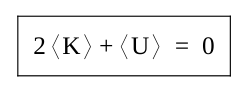
The virial theorem is a fundamental analytical result in the mechanics of particle systems, as it establishes a rigorous connection between the time averages of kinetic and potential energies. Its validity extends to systems in dynamic equilibrium, where internal forces are governed by potentials that depend on distance according to a power law, as in the case of universal gravitation or electrostatics.
The work is written in italian.

pdf_ita Brussi 2026_Il teorema del viriale e l’equilibrio stellare

Teorema del viriale

please, rate this post

Mie scattering and white clouds

Why are clouds white?
We need to examine a type of scattering that involves photons of solar radiation when they interact with the molecules that make up the tiny droplets (or water droplets) forming clouds or fog. Unlike Rayleigh scattering (which involves nitrogen and oxygen molecules in the air, see my post The Rayleigh scattering and the blue sky, whose sizes are smaller than the wavelength of the incoming radiation), in this case the droplets are of the same order of magnitude as the radiation wavelength (or slightly larger). This phenomenon is called Mie scattering, named after the German physicist Gustav Adolf Fedor Wilhelm Ludwig Mie (1869–1957), who provided a rigorous mathematical demonstration of it.

Because these microdroplets are ‘large’, they scatter nearly all wavelengths with approximately the same intensity, so the light appears white (or whitish). There is no wavelength-selection effect as in the case of the blue sky.
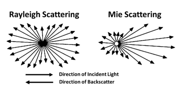
Another characteristic is that the scattering does not occur uniformly in all directions but mainly forward (in the same direction as the incoming light), creating strong glare, while a smaller fraction is scattered backward. See Figure 2.


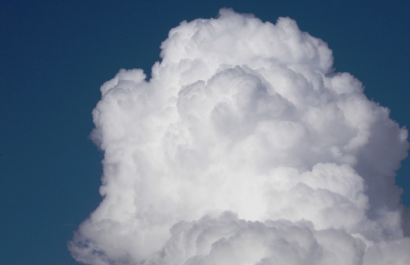
Figure 1 – White clouds !

White clouds


Figure 2 – Rayleigh scattering and Mie scattering

Mie scattering


This explains why clouds tend to be white and why, when you shine car headlights into fog, a blinding glow is produced (due mainly to the backscattered component), see Figure 3. It also explains why truck drivers -whose driving position is at least a couple of meters higher than the level of their headlights (rather than about half a meter or less, as in cars)- experience this backscattering effect to a lesser extent and therefore can actually see the road in fog better than a car driver. See Figure 4 (clearly rather banal examples, only ‘evocative’ to suggest points of view).
This is also the reason why fog lights are always mounted very low, both on cars and on commercial vehicles: to maximize the angle relative to the backscattered glare produced by Mie scattering.


Figure 3 – Blinding glow while driving a car in the fog

Car driving in the fog


Figure 4 – Driving a truck at night

Truck driving


Technically,
Mie theory provides an exact solution to Maxwell’s equations for the interaction of a plane electromagnetic wave with a homogeneous sphere of dielectric material. It has no limits beyond the size of the interacting material (as in the case of Rayleigh scattering).
In Mie theory, the total extinction of light (absorption + scattering) is defined by the coefficient Qₑₓₜ.
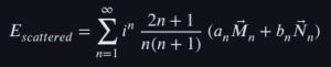
Mathematically, the diffuse electric field is expressed as an infinite series of coefficients (called aₙ and bₙ), which represent the contributions of the electric and magnetic multipoles:
Mie scattering maths
where Mₙ and Nₙ are spherical vector wave functions. The larger the particle (i.e. the fog), the more terms in the series are needed to calculate the correct scattering.

please, rate this post