Post – Page 5 – Andrea Brussi

Understanding the Sizes : 2 – Solar System

Second episode of the deep dives into the measurements of the universe around us. The first one was about the Earth and the Moon.
This one is about the Solar System, that is, the bodies that orbit the Sun, our star.

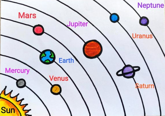
The planets classified as such are, in order of increasing orbital radius: Mercury, Venus, Earth, Mars, Jupiter, Saturn, Uranus, Neptune (see Figure 1). Besides these main bodies there are many secondary ones, such as dwarf planet, moons, asteroids, and comets, but we will focus only on the main objects.

Figure 1 – drawing of the sequence of planets of the solar system

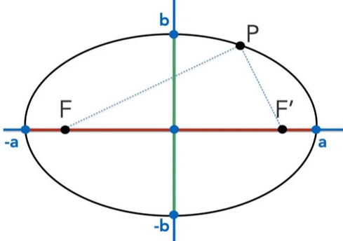
Since Kepler (1571–1630) we know that orbits are ellipses (see Figure 2), with the Sun located at one of the foci. In reality, eccentricity (i.e. a – b with reference to Figure 2) is quite low, about 3% for Earth and modest for all the planets except Mercury. Other celestial bodies orbiting in the Solar System, such as asteroids (larger ‘rocks’ measuring a few hundred kilometers), also exhibit significant eccentricity (which measures how much their orbit deviates from a circle). For simplicity we will consider circular orbits and a single radius.

Figure 2 – An ellipse is a plane curve surrounding two focal points, such that for all points on the curve, the sum of both distances to the two focal points is a constant ( FP + PF’ = constant for each P on the curve); in this example, the eccentricity is very large, while for the planets it is much smaller; the F points are called foci, a is the semi-major axis, b is the semi-minor axis.

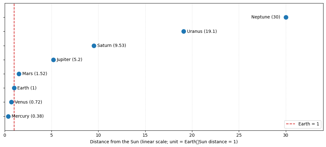
We will not list all of the measurements for these objects, but only a few reference ones. It is important to understand the need to change the reference scale, moving to a larger one, we can no longer use the soccer ball from the previous post. Now let us imagine Earth as a tiny grain of fine sand (0.09 mm), and its distance from the Sun as 1 meter (the radius of its orbit, usually called the astronomical unit, AU). On this scale, the planet closest to the Sun is Mercury (with a radius 0.38 that of Earth), at about 38 cm. Mars (with a radius 0.52 that of Earth) orbits at about 1.5 m; the gas giants Jupiter (radius 11 times that of Earth, i.e., 0.9 mm on the adopted scale) at about 5 m, and Saturn (radius 9.5 times that of Earth) at about 9.5 m. Uranus and Neptune are very far away, at about 19 m and 30 m respectively. See Figure 3 for a scale diagram.

Figure 3 – a scale diagram of distances in the Solar System

But what does this one meter of distance, taken as a reference for Earth’s orbit, correspond to? It is about 149 million km, a distance that would take roughly 170 years to cover by car traveling at 100 km/h. Light, which travels at 300,000 km/s (more than 1 billion km/h), takes about 8 minutes to go from the Sun to Earth, and more than 4 hours to reach Neptune.
And how big is the Sun? Its radius is about 670,000 km, so compared with the Earth as a soccer ball model, it would be a sphere with a radius of 11.60 m, roughly the volume of a a five-story building of 400 square meters per floor. Compared with the Earth as a grain of fine sand model, it would be a ‘grain’ of almost 1 cm (9.3 mm).

Earth has one large moon, the Moon; Mars has two small ones, Phobos and Deimos. Jupiter has four major moons (Io, Europa, Ganymede, Callisto, discovered in 1609 by Galileo Galilei, 1564–1642) and 91 smaller ones. Saturn has as many as 146 in total! Practically all moons are in synchronous rotation, meaning they always show the same face to their planet, like our Moon.

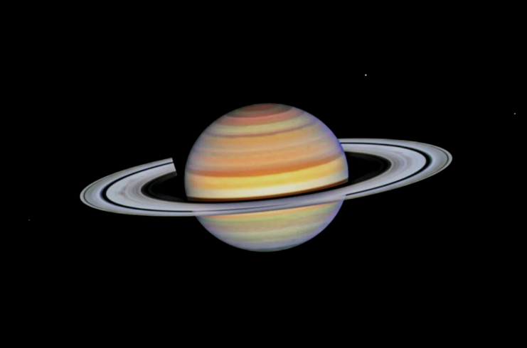
Saturn’s rings (Figure 4), made up of countless particles of ice and rock, are more than 30,000 km wide (three times Earth’s diameter) but extremely thin, ranging from a few tens of meters to a few hundreds of meters. For this reason, when they are seen edge-on (about every 15 Earth years), they reflect almost no sunlight and are not visible from Earth.

Figure 4 – Saturn photo by HST (source: NASA, ESA, STScI, Amy Simon NASA-GSFC)

Beyond the orbit of Neptune, or on our scale between 30 and 50 meters, lies the Kuiper Belt (named after Gerrit Pieter Kuiper, 1905-1973), which contains thousands of icy bodies, remnants of the formation of the Solar System, including dwarf planets like Pluto, essentially distributed in a volume squashed on the plane of the ecliptic. The so-called heliosphere ends here. An even more external region, the Oort Cloud (named after Jan Oort, 1900-1992), between 2 and 200 km on our scale, has been hypothesized to contain an immense diffusion of ice and rocks, the reservoir from which comets are drawn by the Sun. We can consider it as the outer boundary of the Solar System.

Next episodes:
Understanding the Sizes : 3 – Milky Way
Understanding the Sizes : 4 – galaxy clusters and beyond

Previous episode:
Understanding the Sizes : 1 – Earth and Moon

please, rate this post

Understanding the Sizes : 1 – Earth and Moon

In everyday life, we don’t stop to think about the ‘sizes’ of the planet we live in, the Solar System, and the galaxy (Milky Way) in which we orbit with our mothership, Earth.
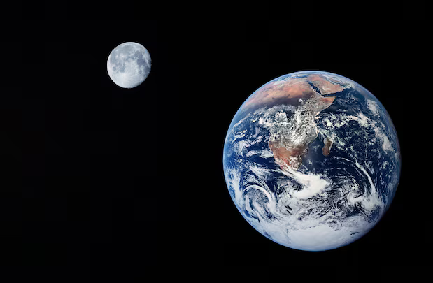
In a series of insights, we aim to understand the distances and some parameters that characterize these systems. This first one concerns the Earth and its satellite, the Moon (Figure 1).

Figure 1 -the Earth and the Moon

The average radius of the Earth (slightly smaller at the poles than at the equator) is approximately 6,370 km, meaning its circumference is approximately 40,000 km. Therefore, an electromagnetic signal traveling at 300,000 km/s would circle the planet 7.5 times in one second.

Here are some interesting measurements to compare:

– The thickness of the troposphere, where virtually all meteorological phenomena occur and almost all water vapor is concentrated, varies from about 8 km (at the poles) to about 20 km (at the equator), or, on average, 14 km. That is, if the Earth were the size of a soccer ball (radius about 11 cm), the troposphere would be roughly the thickness of two sheets of paper (about 0.24 mm).

– The highest mountain (Everest, about 8.8 km) and the deepest ocean (Mariana Trench, about 10.9 km) are of the same order of magnitude as the height of the troposphere. As if to say that if you held that soccer ball in your hand you would almost not notice their presence.

– The Moon, which has a radius of 1,737 km, would be slightly smaller than a tennis ball (radius about 3 cm) compared to the soccer ball sized Earth, see Figure 2. Its average distance from Earth is about 380,000 km, so an electromagnetic signal takes about 1.3 seconds to arrive; in the proportions calculated for the balls, the distance between them would be about 6.5 meters.

Figure 2 – Soccer ball and tennis ball in the proportions of Earth and Moon

– The altitude at which airliners fly, about 10 km, is little more than the thickness of a sheet of paper. Seen from space they appear to crawl more than fly. The International Space Station (ISS) is maintained at an altitude of about 400 km, about 7 mm above the soccer ball, at a speed of about 28,000 km/h, or it would move about 8 mm per minute.

– Considering the Earth’s rotation in 24 hours, the tangential velocity of a point at the equator is almost 1,700 km/h; at our latitudes of about 45°, the speed is just under 1,200 km/h. For this reason, spacecraft launch pads are positioned at low latitudes, near the equator, to take advantage of the higher linear velocity. The escape velocity required to overcome gravitational pull (about 40,000 km/h on Earth) is more easily achieved by exploiting the velocity of the launch point (with a starting direction toward the east for maximum effect, considering that the Earth rotates towards the east and the speeds can add up).
Note that escape velocity is not tied to ‘up’; it’s the minimum speed at a given altitude to be unbound, in any direction, as long as you don’t collide with the planet.

Next episodes:
Understanding the Sizes : 2 – Solar System
Understanding the Sizes : 3 – Milky Way
Understanding the Sizes : 4 – galaxy clusters and beyond

please, rate this post

How empty is matter?

Very empty.
Extremely empty.

Let’s consider the elementary constituents, atoms, which then aggregate into molecules to form the matter we know. They consist of a nucleus that represents almost the entire mass, in the form of positively charged protons and neutrons with almost equal mass to protons but without charge, and very light (1/2000 the mass of the proton) negatively charged electrons that ‘orbit’ around the nucleus. Under normal conditions, the electric charges of the protons and electrons of the ‘neutral’ atom balance each other out. All aggregations between atoms occur thanks to the forces of attraction between different charges, whereas, as we know, equal charges repel each other, as is the case with magnetic forces. In the nucleus, protons, although they have the same positive charge and repel each other, are held together by an extremely strong force called the strong nuclear force.

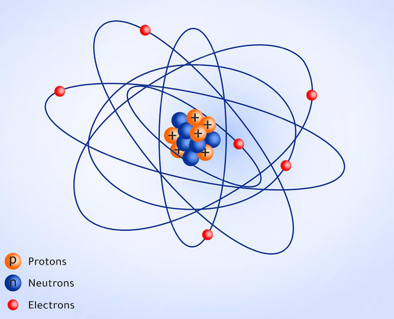
Figure 1 – example of a very imprecise diagram of an atom (source: freepic.com)

Figure 1 is a typical example of a misrepresentation of an atom, for many reasons, but two are primary: the particles are not ‘balls’ but probability densities, that is, ‘elongated clouds’ rather than ‘balls’; the proportions are monstrously misleading.
This brings us to the topic of this post.
Let’s consider the smallest and simplest atom, the neutral hydrogen atom H (consisting of 1 proton and 1 electron), and the neutral iron atom Fe (the most common isotope is composed of 26 protons, 30 neutrons and 26 electrons). The mass of Fe is therefore about 56 times that of H.
For atomic measurements, we use angstroms (Å, named after the Swedish physicist Anders Jonas Ångström, 1814-1874), equal to one-tenth of a billionth of a meter (10¯¹º m).
We also consider only the nuclei and the minimum distance of the electrons from the nucleus, that is, the radius of their innermost orbit (so the ‘size’ of the entire atom is much larger).
Some actual measurements of these particles are approximately as follows:

Atom	Nucleus	Min distance electrons	Δ
H	1,7 · 10^-5 Å (0,000017 Å)	0,5 Å	~2.9 · 10⁴
Fe	5 · 10^-5 Å (0,00005 Å)	1,25 Å	~2.5 · 10⁴

So between the nucleus and the innermost orbit of the electrons there are about four orders of magnitude! This is empty space. Obviously, there are electric fields holding everything together, but there are no massive particles, bound or not, in that space, and there can’t be any in any atom, under normal conditions of matter.

Four orders of magnitude means that if the Fe nucleus were the size of a plum (5 cm), there would be empty space up to 1250 meters away. For H, if the nucleus were the size of a grape (17 mm), there would be empty space up to 500 meters away.

What allows matter to be bound in the solid state are the electrical binding forces between atoms, due to the presence/absence of electrons in outermost atomic shells, but that’s another story.
These empty spaces compress only under extreme conditions, for example when matter degenerates in stars that transform into white dwarfs or neutron stars (when the outward force of radiation ceases and gravity compresses the star), reaching unimaginable densities (a grape would have a mass of billions of tons). But that’s another story, too.

please, rate this post

Olbers’ paradox and the dark night sky

Why is the night sky dark?
If universe were infinite, eternal, and static, as Giordano Bruno (1548-1600) claimed, as did cosmology until the early 20th century, adding that it is also populated by stars in a homogeneous manner, the night sky should be bright and not dark. This contradiction was already noted by Johannes Kepler (1571-1630) in 1610 in Dissertatio cum Nuncio Sidereo.
However, the principle was clearly formulated in 1826 by Einrich Wilhelm Olbers (1758-1840), who mathematically demonstrated (see below, optional reasoning which can be skipped) why the night sky should shine according to the cosmology of the time, highlighting a paradox with respect to observation.

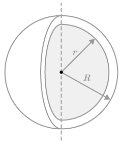
Imagining the universe as consisting of spherical shells concentric with respect to our point of observation (see Figure 1), the intensity of radiation received (flux f ) from a source ( L ) at a distance ( r ) is inversely proportional to the square of the distance:
[1] f = L / 4 π r²
The number of sources contained in the shell is proportional to the volume, which increases with the square of the distance (by infinitesimal increments
dr = R – r with reference to Figure 1):
[2] dn ∝ dV ≈ 4 π r² dr
Therefore, the effects of [1] and [2] compensate each other and each shell contributes with the same intensity, regardless of distance.
The infinitesimal intensity ( dI ) coming from the infinitesimal shell, multiplying [1] and [2], is:
[3] dI = f dn = n L dr
Integrating [3] gives the total intensity:
[4] I =∫₀ᴿ n L dr = n L R
Therefore, for R → ∞, the intensity [4] should become infinite. So something is wrong with the reasoning (hence the paradox).

Figure 1 – sketch of a spherical shell

The observation of the dark night sky is explained in modern terms (based on cosmological standard model) because the universe has existed for a finite time (Big Bang hypothesis) and is expanding (interpretation of the redshift of radiation from remote sources).
In the first case, it is considered that the light from remote sources, which has a finite speed, simply has not reached us yet.

In the second case, redshift, or the shift of light towards longer wavelengths (for example, in the infrared band, beyond the range visible to the eye), prevents the observation of remote sources.
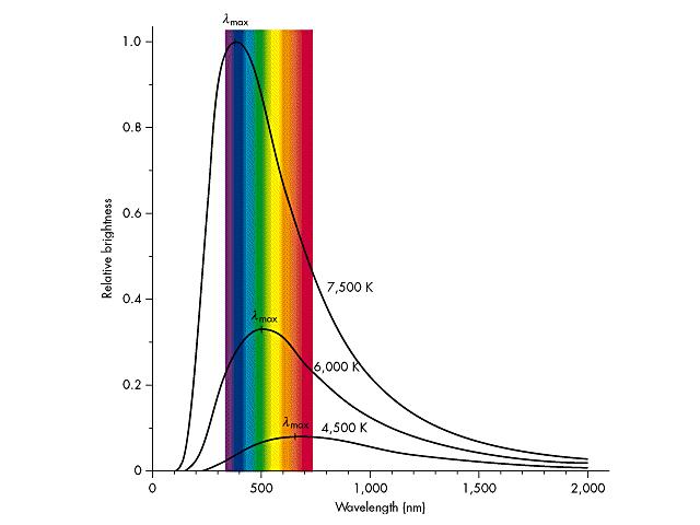
It should also be remembered that the distribution of the intensity of radiation from stellar sources follows a Planckian curve (see Figure 3), which has its maximum in the visible light band. In other words, there are no significant intensities of radiation in a typical stellar source that, moving due to the effect of redshift, could affect this visible band.
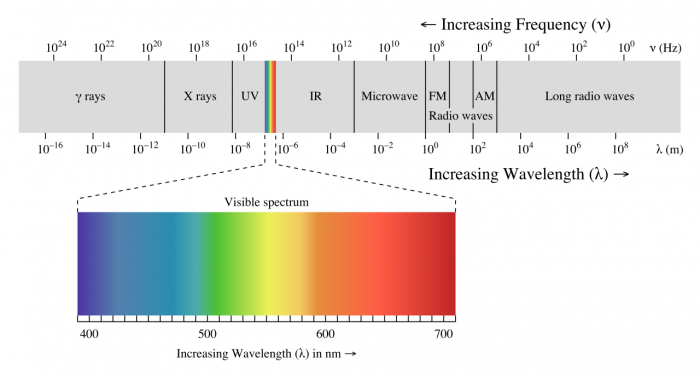
In fact, we emphasize that the range of radiation visible to our eyes is very small compared to the entire spectrum of radiation, as shown in Figure 2.
In reality, redshift alone would explain the dark night sky, even if the universe were infinite and without assuming a Big Bang. And even without expansion, if the observed redshift had a different cause.

Figure 2 – full spectrum of radiation with visible band

Figure 3 – A sketch of a Planckian functions of brightness (intensity of radiation emitted per unit solid angle) for stellar sources with different surface temperatures. That of the Sun is approximately 5700 K.

please, rate this post

The Rayleigh scattering and the blue sky

Why is the daytime sky blue?
We need to examine a type of scattering that affects photons from solar radiation when they interact with the molecules that make up the atmosphere, namely nitrogen and oxygen (99% of the components).
This is Rayleigh scattering (named after Nobel Prize winner John William Strutt Rayleigh, 1842-1919), which affects particles smaller than the wavelength of the incident radiation. It is an elastic scattering, so the wavelength of the same radiation is not changed.
We are dealing with photons, but the formula was developed on the basis of classical electromagnetic theory, not quantum theory (which was created after Rayleigh’s death).

Figure 1 – Angular dependence of Rayleigh Scattering
(copyright MLisandra, CC BY-SA 4.0, via Wikimedia Commons, here without the formula inscription)

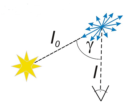
For the explanation we are looking for, the Rayleigh scattering formula can be simplified as follows (see also Figure 1):
[1] I ~ I₀ (1+cos²γ) / λ⁴
where I is the intensity of the scattered radiation, I₀ is the intensity of the incident radiation with wavelength λ , γ is the scattering angle of the incident radiation.

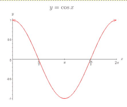
We can immediately see that the angle where the intensity [1] is lowest is the right angle ( π/2 ), where the cosine is zero (see Figure 2), meaning that the sky is darkest (the blue is most intense) at an angle of 90° to the direction of the Sun.
Furthermore, the dependence on the inverse of the fourth power of λ suggests that the effects for different wavelengths are significantly different. In fact, blue light is scattered much more than red light, which has a longer wavelength (see Figure 3), making the sky blue. Even shorter wavelengths, such as those of violet, are less intense at source and do not contribute significantly.
At dawn and dusk, blue light is highly scattered by the greater layer of atmosphere it passes through, together with yellow and green light, so red/orange light dominates.

In the case of smaller particles, the cross section and refractive index of the particle are considered, but even if atmospheric gas molecules are treated as point sources, in this case the effects depend on their polarizability due to incident radiation. Those who take photographs using a polarizing filter are familiar with this phenomenon: in fact, by adjusting the filter effect and therefore the polarization, the sky can even become completely black at 90° to the Sun, which can be creative but not very realistic!

Figure 2 – cosine function behaviour

Figure 3 – visible band of radiation

See also Mie scattering and white clouds.

please, rate this post

Eddington luminosity and limits to stellar growth

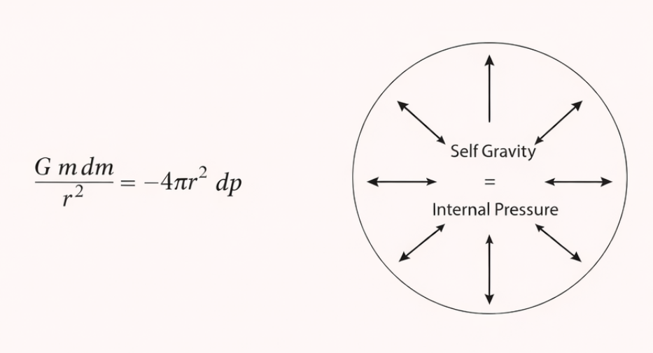
The Eddington luminosity (Lₑ) (named after Arthur Stanley Eddington, 1882-1944), also known as the Eddington limit, is the growth limit of a structure that is in hydrostatic equilibrium (see Figure 1), balancing the outward radiation pressure with the inward gravitational pull.

Figure 1 – Hydrostatic equilibrium

The relationship for the luminosity limit can be easily derived, obtaining:
[1] L ≤ 4π c G M / k = Lₑ
where G is the universal gravitational constant, M is the mass of the object, c is the speed of light, and k is the opacity (ability to absorb radiation) of the material that makes up the object.
As a function of solar parameters, in the case of the model consisting of ionized hydrogen, [1] can be expressed as:
[2] Lₑ ≈ 3.2 * 10⁴ (M/M๏) L๏
where M๏ and L๏ are the mass and luminosity of the Sun.

In the very hot core of massive stars (or in accretion disks of black holes), opacity is independent of frequency and temperature, is related to Thomson scattering (see Thomson scattering on Wikipedia for more informations) of free electrons, and can be expressed as:
[3] kₑₛ = σₜ nₑ / ρ
where σₜ is the Thomson cross section for electrons, nₑ is the number density of electrons, and ρ is the density of the medium.
To consider the more general case of models also consisting of helium and metals, the general relationship is expressed as a function of the mass fraction (X) of hydrogen, and the [3] becomes:
[4] kₑₛ = σₜ (1+X) / 2 mₚ ≈ 0.2 (1+X) cm² / gr
where mₚ is the mass of the proton.
Therefore, in the case of a model consisting only of helium, Eddington luminosity would double (with X=0 , [4] is halved and [1] is doubled).
Relationships can also be derived for cases of models that are not fully ionized or colder (for less massive stars), or for highly energetic radiation (e.g., gamma rays as in black hole accretion disks), but these are beyond the scope of this note.

What is notable is that this physical limit explains why we do not observe infinitely large stars; beyond a certain mass limit, the luminosity is such that it disrupts the star.
The Eddington luminosity also defines the maximum rate at which a black hole can grow: if matter falls too quickly, the light emitted repels it back.

please, rate this post

A sharp presentation of a quantum mechanics course

Not all professors are so explicit in presenting a quantum mechanics course, which is objectively very challenging. A medal for intellectual honesty to this professor!
(yes, it’s an old video, but it’s still worth watching ; )

Presentation of a quantum mechanics course

please, rate this post

Sabine on gauge symmetry and light

An interesting talk by Sabine Hossenfelder that visualizes gauge symmetry with an effective metaphor, associated with the existence of electrons and electromagnetic radiation.

please, rate this post

Snell’s law and the causes of refraction

Let us recall Snell’s well-known law, which describes the phenomenon of refraction:
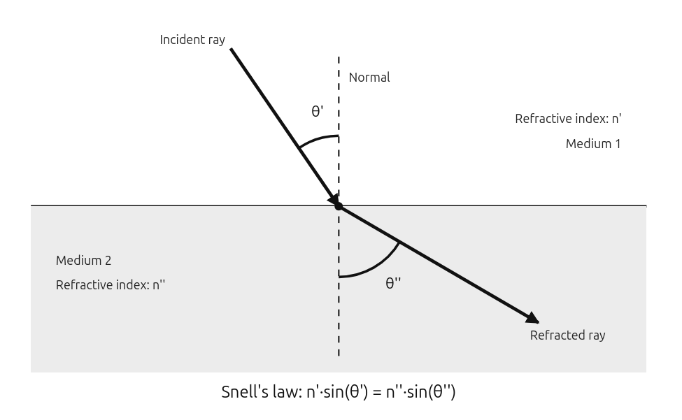
– a ray of light undergoes a deviation when it passes from one transparent medium to another with a different refractive index (see Figure 2).

Figure 1 – Snell law

Figure 2 – Refraction example

Mathematically (see Figure 1):
[1] n’ sin(θ’) = n” sin(θ”)
where n’ , n” are the refractive indices of the two transparent media, θ’ , θ” are the angles of incidence and refraction (measured relative to normal at the interface between the media).
In other words, given two media, the ratio between the respective sines of the angles of incidence and refraction is constant.
A first proof can be obtained by applying Pierre de Fermat’s (1601-1665) principle of least time, namely that light follows the path that requires the least time to travel from one point to another. Attached below is the simple geometric-analytical proof (in italian):

Fermat_Snell_geometric-analytical demonstration

Okay, this relationship (perhaps already studied in the 10th century by the Persian mathematician Ibn Sahl) is certainly interesting, but what is the physical motivation for this constant quantity? It is necessary to identify where this regularity lies.
The reasons derive directly from Maxwell’s equations, the fundamental laws describing the interaction between electric and magnetic fields.
From these, it follows that the boundary conditions require that the tangential components of the electric field and magnetic field be continuous across the separation surface. Therefore, the phase of the incident, (reflected,) and transmitted wave must be the same along this boundary.

The assumption that the frequency ( ν ) of the incident light remains constant (i.e., that it is independent of the medium in which it propagates) can also be understood by considering that if this were not the case, it would lose coherence as it crossed the surface between the two media, probably transforming the image observed through the separation surface into a uniform grey color, which is not observed.
Furthermore, since the energy associated with incident photons is E = h ν , where h is the Planck constant, the same conservation of energy tells us that the frequency cannot change.
Quantistic note: this consideration refers to a single photon, which would change color (towards red) if it lost energy (phenomenon that does not occur for all observed refracted photons). Considering a beam of photons, however, it may be that the second medium causes absorption of the incident light, thus a decrease in total energy, but this concerns the entire beam that absorbs some photons completely and not the individual photons.

Considering the wave vectors k’ (incident) and k” (refracted) associated with their respective phases, and equating their projections on the separation interface, we obtain:
[2] k’ sin(θ’) = k” sin(θ”)
but k = ω / v , where ω is the angular frequency of the electromagnetic wave of the incident light, v is the velocity in the medium, and defining the refractive index n = c / v (derived from the constants ε₀ and μ₀ of the medium using Maxwell’s equations, where c = 1/√(ε₀ μ₀) ), from [2] we finally obtain [1] .

please, rate this post

The three-body problem and the five Lagrangian points

Joseph-Louis Lagrange (1736-1813) was a great mathematician of the 18th century. His main studies on mechanics led him to tackle the gravitational three-body problem, which, however, remains unsolved to this day because the system is inherently chaotic and unpredictable in the long term, as small initial variations cause drastically different results.
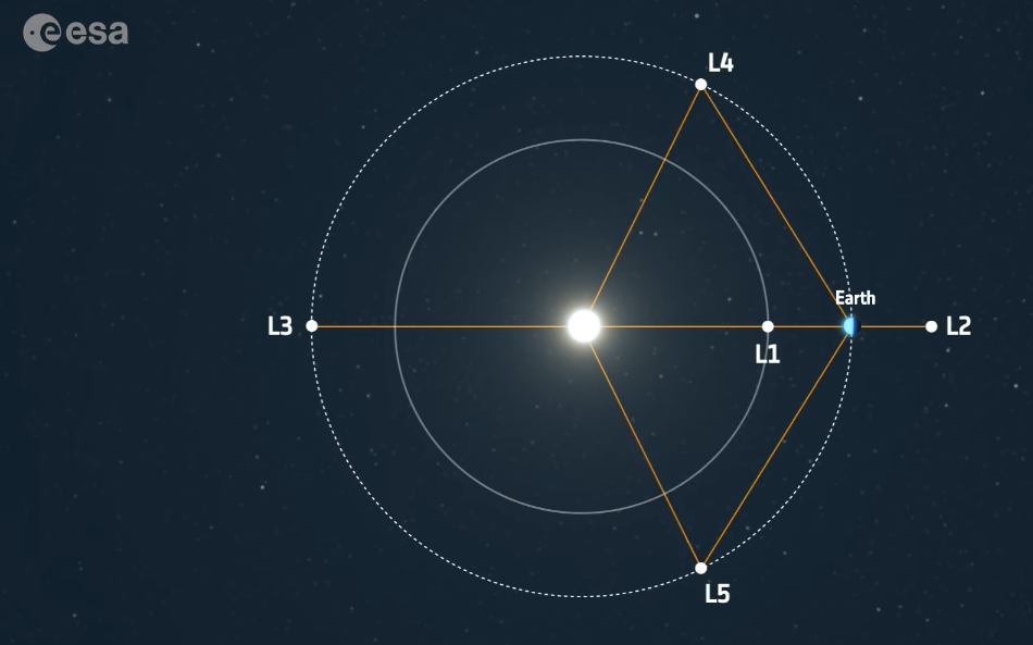
Lagrange found the equilibrium solutions (the five Lagrangian points, see figure taken from the ESA website) for the system in the simplified yet highly interesting case where the third body has negligible mass compared to the other two (e.g., the Sun, a planet, and an asteroid or an artificial satellite). The first three points (L1, L2, L3) had already been found by Leonhard Euler (1707-1783), another huge mathematician of the 18th century, while Lagrange found the so-called ‘triangular’ points (L4, L5), because they form perfect equilateral triangles with the two main bodies.
For details about these points, please refer to the easy explanations on the
ESA (European Space Agency) website.

Obviously, Lagrange could never have known about the evidence supporting his conjecture (it was only in 1906 that astronomers confirmed his theory by discovering Trojan asteroids captured at points L4 and L5 of Jupiter’s orbit) or its current usefulness in positioning our space exploration vehicles.
Thanks to their ‘gravitational stability’, which saves positioning energy (and in the case of L2 also provides partial shielding from the Sun), it is conceivable that, in the future of space exploration, advanced bases for deep space exploration will be located at Lagrangian points.

The 5 Lagrangian points, from the ESA (European Space Agency) website; the orbits of points L1 and L2 are not to scale, the distance from Earth is about 1/100 of the radius of Earth’s orbit.

please, rate this post