Understanding the Sizes : 4 – galaxy clusters and beyond

Exploring beyond our galaxy, to be able to reach the edges of the known universe with measurements that can be perceived, it is necessary to change scale again compared with the previous post on the Milky Way. Over there, the distances involved become almost impossible to truly understand, they are so mindblowing!

Let us now consider our galaxy to be 1 millimeter across. We are part of a ‘local’ group of galaxies made up of more than a hundred smaller galaxies (of which only one is of significant size, the Triangulum Galaxy, known as M33, see Figure 1), and a large spiral galaxy broadly similar to ours, Andromeda (Figure 2), which is about 2.5 cm away. Andromeda is the most distant cosmological object that can be seen with the naked eye (see also my post References for laymen: angles in the sky).


Figure 1 – triangle galaxy M33 (credits: Nasa, Esa e M. Durbin, J. Dalcanton e B. F. Williams, University of Washington)
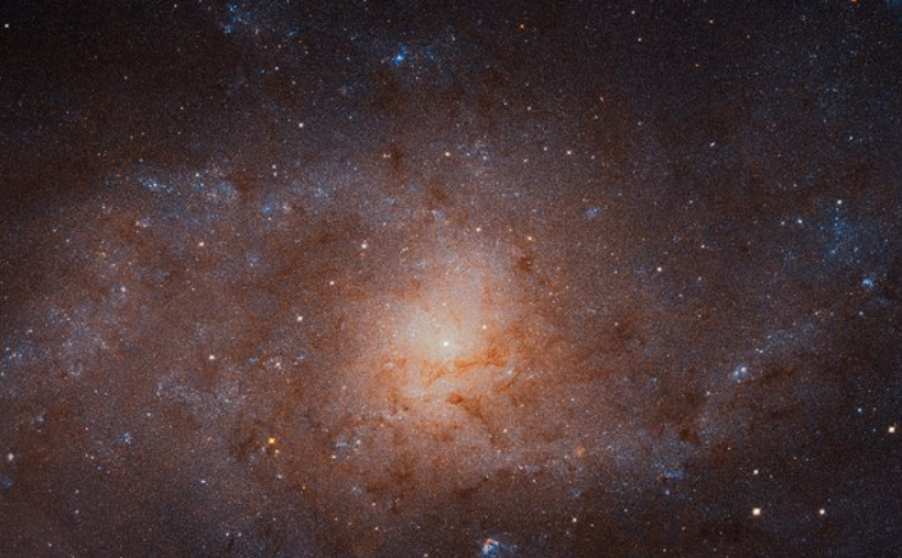
Triangle galaxy M33


Figure 2 – Andromeda galaxy (image credit: Westend61 via Getty Images)
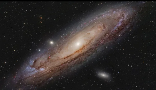

Andromeda is more extended but less massive than our galaxy. It’s getting closer to us (or rather we’re getting closer to each other) at about 400,000 km/h, on our new scale, less than four thousandths of a millimeter (about one hundredth the thickness of a hair) in a million years. In other words, in 4–5 billion years the two galaxies will merge, still in a collisionless way (we demonstrated this here, §1, not for newbies), and will probably turn into a giant elliptical galaxy (like NGC 1600 in Figure 3) after a few more billion years. However, recent measurements from the Gaia* satellite reduce the probability of this merger happening on such ‘short’ timescales, even though it is inevitable that it will occur.

* The Gaia satellite is an astrometric mission of the European Space Agency (ESA), launched in 2013 to map the Milky Way in 3D. It orbits around the Lagrange point L2 (see my post The three-body problem and the five Lagrangian points), and has created the most precise stellar catalog of more than 2 billion stars around us, measuring their positions, motions, brightness, and chemical composition.


Figure 3 – NGC 1600 by HST, it has a diameter of about 120.000 light -years, or about 1.2 mm on our scale (credits: A. Quillen, University of Rochester, G. Bower, CSC/STScI, and G. Rieke, Steward Observatory/University of Arizona)
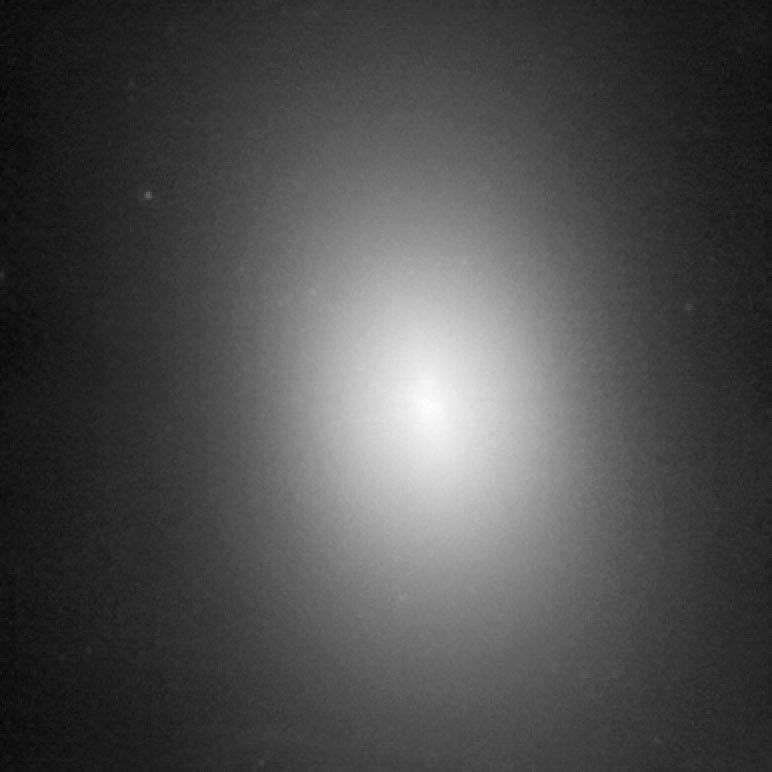
NGC 1600


The Local Group of galaxies (see the 3D schematic in Figure 4) has a radius of about 3 cm on the adopted scale, and is surrounded in an “homogeneous” way by similar structures. For example, in Figure 5 a radius of 33 cm is considered on the same scale, and in Figure 6 a radius of about 1.5 m. Proceeding in an analogous way, one can reach the limit of the observable universe (that is, before redshift completely prevents sources from being detected) which, on the adopted scale, can be taken to be at a distance of just over 4 meters.


Figure 4 – Local Group of galaxies (source starwalk.space)
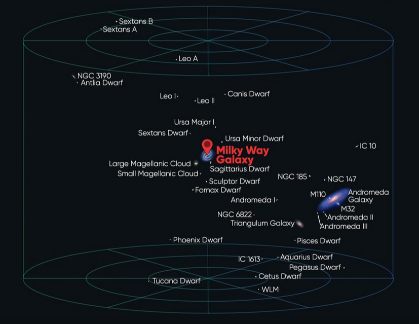
local galaxies cluster


Figure 5 – Virgo Supercluster, along with 100 other galaxy groups (source starwalk.space)
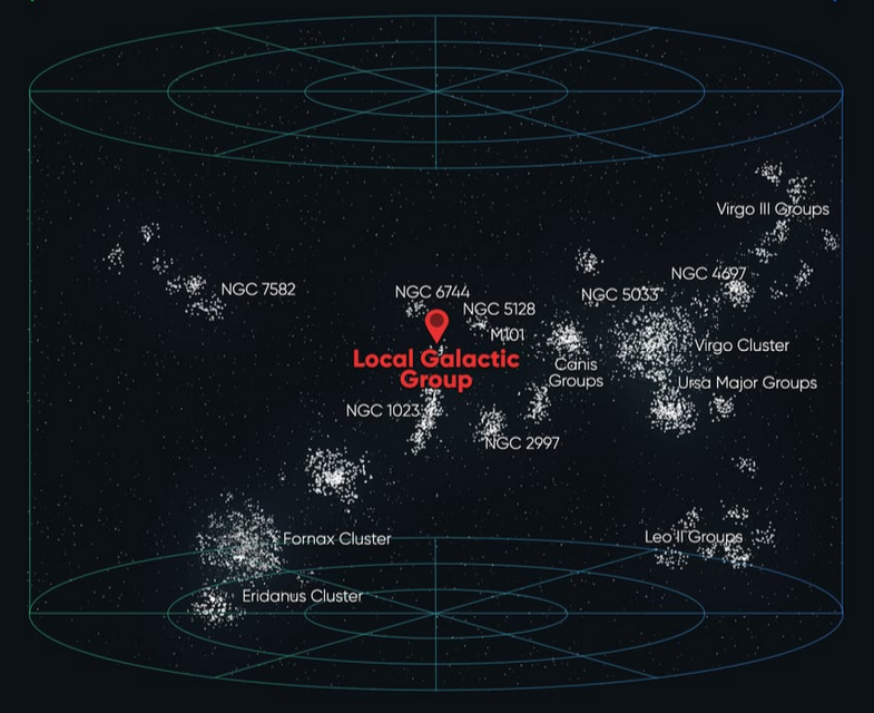
Virgo Supercluster


Figure 6 – Laniakea Supercluster which includes almost 100.000 galaxies more than ours (source starwalk.space)
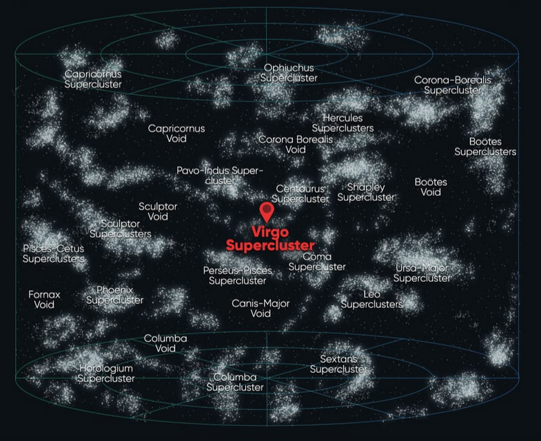
Super Supercluster


We have reached the limit of the current theory of the standard cosmological model. It is a theory, based on creation from nothing through an initial Big Bang, which is strongly supported by observations but also has major gaps in explaining other evidence.
Our journey therefore stops right at the limit of ‘measurable’ findings grounded in commonly accepted theories; beyond this point, it becomes epistemology rather than cosmology.


Previous episodes:
Understanding the Sizes : 3 – Milky Way
Understanding the Sizes : 2 – Solar System
Understanding the Sizes : 1 – Earth and Moon
please, rate this post

Understanding the Sizes : 3 – Milky Way

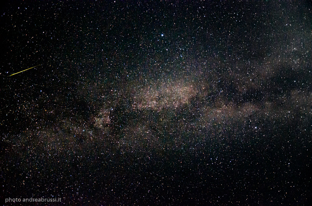
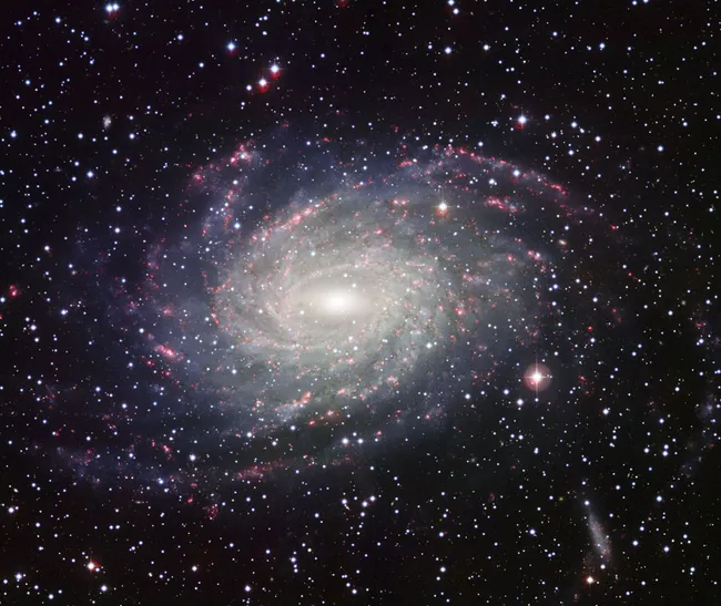
The Milky Way is our galaxy: a gravitationally bound structure that includes about 100 billion stars and an enormous amount of gas (essentially atomic hydrogen), with an approximate shape of a rotating disk, which, of course, we can only imagine and not actually see, since we are inside it (our view towards the galactic centre is known, see Figure 1, even if it is increasingly difficult to observe, due to atmospheric pollution, especially light pollution.). See Figure 2 for a photo of a similar example. The stars, gas, and dust that make up the disk rotate in the sense that they orbit around the roughly spherical central nucleus (the bulge), which instead is not rotating (its stars have chaotic motions).


Figure 1 -Milky Way as seen from Earth (my photo)

Milky Way


Figure 2 – example of a galaxy similar to the Milky Way: NGC 6744, taken at the European Southern Observatory’s La Silla Observatory in Chile (image credits: ESO)

Galaxy like Milky Way


To understand the sizes, it is necessary to change scale again compared with the previous post on the Solar System: the quantities involved become increasingly difficult to ‘grasp’. We have seen that Sun light takes about 4 hours to reach Neptune, the outermost planet of the Solar System. The star closest to us is Proxima Centauri (a red dwarf in a triple star system), about 4 light-years away. We therefore choose the light-year as the unit for this new distance scale, imagining 1 light-year as equal to 1 millimeter. Then Proxima Centauri is about 4 mm from the Sun (of course, since the difference is only a few light-minutes compared with 4 light-years, Earth and the Sun that Earth orbits can be considered at essentially the same distance).

All these stars orbit around the nucleus but also have their own independent motions, which are collisionless (we demonstrated this here, §1, not for newbies), a remarkable fact given the number of bodies, and in contrast, for example, with a collection of gas molecules in a container, which instead undergo continuous collisions (which determine its pressure and temperature). But compared with a gas, the distances between the components in a galaxy are immensely larger.

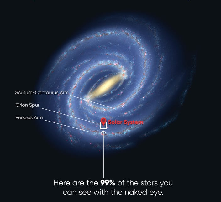
In the new scale we have adopted, the radius of the galactic disk is about 105 meters (about 105,000 light-years), and our position is about 26 meters from the center. In Figure 3 the drawing schematically outlines one possible configuration and the proportions. Our linear speed is about 790,000 km/h and we complete one orbit in about 250 million years, so on our scale, despite the crazy speed, we move only about 1.5 cm in a thousand years, in this 105-meter-radius disk. Since the Sun and Earth formed, about 4.5 billion years ago, we have made about 18 revolutions around the galactic nucleus.


Figure 3 – schematic drawing of the Milky Way and its proportions (gases beyond the star limit are not drawn but they are gravitationally relevant; source starwalk.space)

MIlky Way sketch


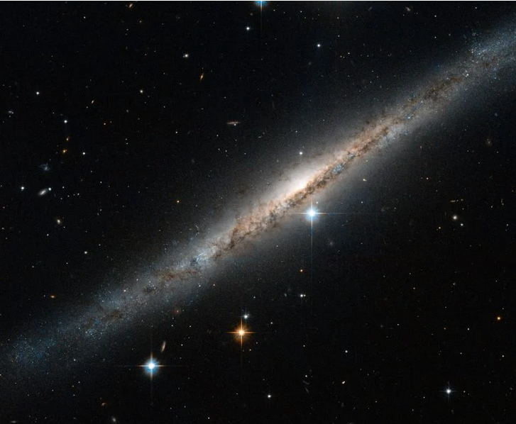
The disk of our galaxy is made up of several arms, where the concentration of stars is higher, and a more rectilinear component that originates from the central nucleus, from which the arms branch out, as schematized in Figure 3. A galaxy of this kind is called a ‘barred spiral’ and its shape when seen edge-on is similar to the example in Figure 4.
In a future post we will talk about the central black hole and the star-forming regions.


Figure 4 – Example of a spiral galaxy seen edge-on, ESO 121-6 (source: HST by ESA/Hubble & NASA)

Galaxy edge on Eso121-6


As a final remark, note that nearly all the stars visible to the naked eye belong to the Sun’s local stellar neighborhood, as highlighted in Figure 3. It’s a tiny region compared with the size of the whole Milky Way. Most of the Galaxy’s other stars are too faint and/or too obscured by interstellar dust to be seen individually, and instead contribute to the Milky Way’s diffuse glow: a blend of millions to billions of unresolved stars.


Next episode:
Understanding the Sizes : 4 – galaxy clusters and beyond

Previous episodes:
Understanding the Sizes : 2 – Solar System
Understanding the Sizes : 1 – Earth and Moon
please, rate this post

Understanding the Sizes : 2 – Solar System

Second episode of the deep dives into the measurements of the universe around us. The first one was about the Earth and the Moon.
This one is about the Solar System, that is, the bodies that orbit the Sun, our star.

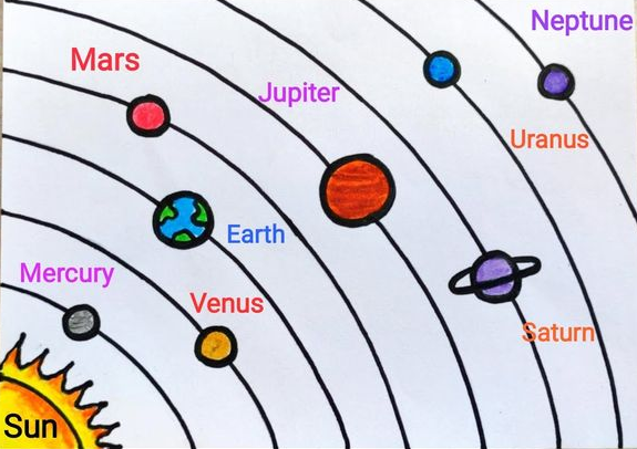
The planets classified as such are, in order of increasing orbital radius: Mercury, Venus, Earth, Mars, Jupiter, Saturn, Uranus, Neptune (see Figure 1). Besides these main bodies there are many secondary ones, such as dwarf planet, moons, asteroids, and comets, but we will focus only on the main objects.


Figure 1 – drawing of the sequence of planets of the solar system

Solar System


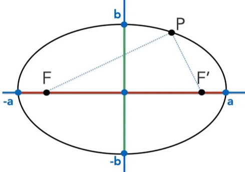
Since Kepler (1571–1630) we know that orbits are ellipses (see Figure 2), with the Sun located at one of the foci. In reality, eccentricity (i.e.  a – b  with reference to Figure 2) is quite low, about 3%  for Earth and modest for all the planets except Mercury. Other celestial bodies orbiting in the Solar System, such as asteroids (larger ‘rocks’ measuring a few hundred kilometers), also exhibit significant eccentricity (which measures how much their orbit deviates from a circle). For simplicity we will consider circular orbits and a single radius.


Figure 2 – An ellipse is a plane curve surrounding two focal points, such that for all points on the curve, the sum of both distances to the two focal points is a constant ( FP + PF’ = constant for each P on the curve); in this example, the eccentricity is very large, while for the planets it is much smaller; the F points are called foci, a is the semi-major axis, b is the semi-minor axis.

Ellipse


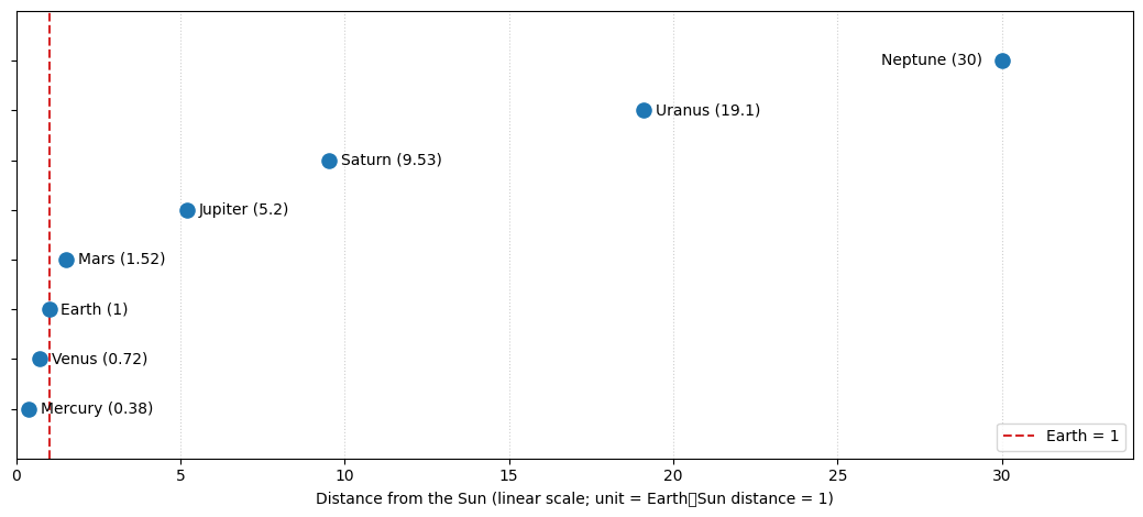
We will not list all of the measurements for these objects, but only a few reference ones. It is important to understand the need to change the reference scale, moving to a larger one, we can no longer use the soccer ball from the previous post. Now let us imagine Earth as a tiny grain of fine sand (0.09 mm), and its distance from the Sun as 1 meter (the radius of its orbit, usually called the astronomical unit, AU).  On this scale, the planet closest to the Sun is Mercury (with a radius 0.38 that of Earth), at about 38 cm. Mars (with a radius 0.52 that of Earth) orbits at about 1.5 m; the gas giants Jupiter (radius 11 times that of Earth, i.e., 0.9 mm on the adopted scale) at about 5 m, and Saturn (radius 9.5 times that of Earth) at about 9.5 m. Uranus and Neptune are very far away, at about 19 m and 30 m respectively. See Figure 3 for a scale diagram.


Figure 3 – a scale diagram of distances in the Solar System

Solar System distances


But what does this one meter of distance, taken as a reference for Earth’s orbit, correspond to? It is about 149 million km, a distance that would take roughly 170 years to cover by car traveling at 100 km/h. Light, which travels at 300,000 km/s (more than 1 billion km/h), takes about 8 minutes to go from the Sun to Earth, and more than 4 hours to reach Neptune.
And how big is the Sun? Its radius is about 670,000 km, so compared with the Earth as a soccer ball model, it would be a sphere with a radius of 11.60 m, roughly the volume of a a five-story building of 400 square meters per floor. Compared with the Earth as a grain of fine sand model, it would be a ‘grain’ of almost 1 cm (9.3 mm).

Earth has one large moon, the Moon; Mars has two small ones, Phobos and Deimos. Jupiter has four major moons (Io, Europa, Ganymede, Callisto, discovered in 1609 by Galileo Galilei, 1564–1642) and 91 smaller ones. Saturn has as many as 146 in total! Practically all moons are in synchronous rotation, meaning they always show the same face to their planet, like our Moon.

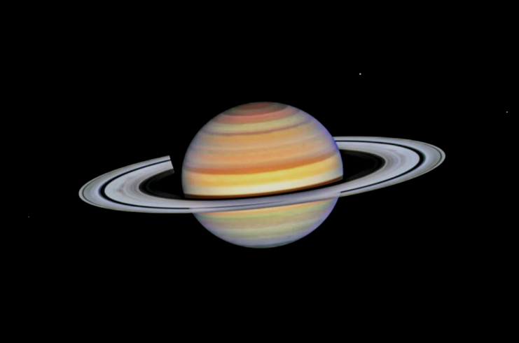
Saturn’s rings (Figure 4), made up of countless particles of ice and rock, are more than 30,000 km wide (three times Earth’s diameter) but extremely thin, ranging from a few tens of meters to a few hundreds of meters. For this reason, when they are seen edge-on (about every 15 Earth years), they reflect almost no sunlight and are not visible from Earth.


Figure 4 – Saturn photo by HST (source: NASA, ESA, STScI, Amy Simon NASA-GSFC)

Saturn


Beyond the orbit of Neptune, or on our scale between 30 and 50 meters, lies the Kuiper Belt (named after Gerrit Pieter Kuiper, 1905-1973), which contains thousands of icy bodies, remnants of the formation of the Solar System, including dwarf planets like Pluto, essentially distributed in a volume squashed on the plane of the ecliptic. The so-called heliosphere ends here. An even more external region, the Oort Cloud (named after Jan Oort, 1900-1992), between 2 and 200 km on our scale, has been hypothesized to contain an immense diffusion of ice and rocks, the reservoir from which comets are drawn by the Sun. We can consider it as the outer boundary of the Solar System.


Next episodes:
Understanding the Sizes : 3 – Milky Way
Understanding the Sizes : 4 – galaxy clusters and beyond

Previous episode:
Understanding the Sizes : 1 – Earth and Moon
please, rate this post

Understanding the Sizes : 1 – Earth and Moon
In everyday life, we don’t stop to think about the ‘sizes’ of the planet we live in, the Solar System, and the galaxy (Milky Way) in which we orbit with our mothership, Earth.
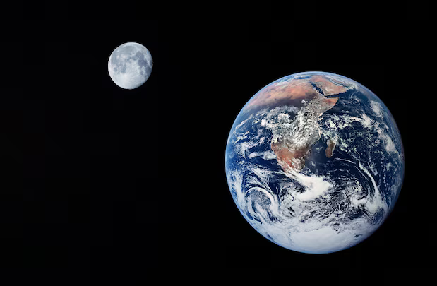
In a series of insights, we aim to understand the distances and some parameters that characterize these systems. This first one concerns the Earth and its satellite, the Moon (Figure 1).


Figure 1 -the Earth and the Moon

Earth_Moon


The average radius of the Earth (slightly smaller at the poles than at the equator) is approximately 6,370 km, meaning its circumference is approximately 40,000 km. Therefore, an electromagnetic signal traveling at 300,000 km/s would circle the planet 7.5 times in one second.

Here are some interesting measurements to compare:

– The thickness of the troposphere, where virtually all meteorological phenomena occur and almost all water vapor is concentrated, varies from about 8 km (at the poles) to about 20 km (at the equator), or, on average, 14 km. That is, if the Earth were the size of a soccer ball (radius about 11 cm), the troposphere would be roughly the thickness of two sheets of paper (about 0.24 mm).

– The highest mountain (Everest, about 8.8 km) and the deepest ocean (Mariana Trench, about 10.9 km) are of the same order of magnitude as the height of the troposphere. As if to say that if you held that soccer ball in your hand you would almost not notice their presence.

– The Moon, which has a radius of 1,737 km, would be slightly smaller than a tennis ball (radius about 3 cm) compared to the soccer ball sized Earth, see Figure 2. Its average distance from Earth is about 380,000 km, so an electromagnetic signal takes about 1.3 seconds to arrive; in the proportions calculated for the balls, the distance between them would be about 6.5 meters.


Figure 2 – Soccer ball and tennis ball in the proportions of Earth and Moon

balls


– The altitude at which airliners fly, about 10 km, is little more than the thickness of a sheet of paper. Seen from space they appear to crawl more than fly. The International Space Station (ISS) is maintained at an altitude of about 400 km, about 7 mm above the soccer ball, at a speed of about 28,000 km/h, or it would move about 8 mm per minute.

– Considering the Earth’s rotation in 24 hours, the tangential velocity of a point at the equator is almost 1,700 km/h; at our latitudes of about 45°, the speed is just under 1,200 km/h. For this reason, spacecraft launch pads are positioned at low latitudes, near the equator, to take advantage of the higher linear velocity. The escape velocity required to overcome gravitational pull (about 40,000 km/h on Earth) is more easily achieved by exploiting the velocity of the launch point (with a starting direction toward the east for maximum effect, considering that the Earth rotates towards the east and the speeds can add up).
Note that escape velocity is not tied to ‘up’; it’s the minimum speed at a given altitude to be unbound, in any direction, as long as you don’t collide with the planet.


Next episodes:
Understanding the Sizes : 2 – Solar System
Understanding the Sizes : 3 – Milky Way
Understanding the Sizes : 4 – galaxy clusters and beyond

please, rate this post

How empty is matter?

Very empty.
Extremely empty.

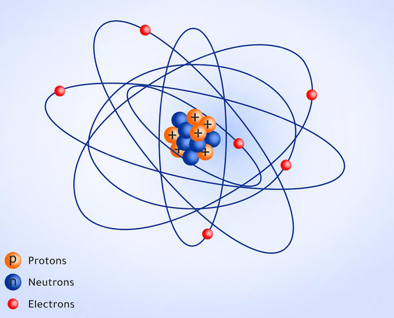
Let’s consider the elementary constituents, atoms, which then aggregate into molecules to form the matter we know. They consist of a nucleus that represents almost the entire mass, in the form of positively charged protons and neutrons with almost equal mass to protons but without charge, and very light (1/2000 the mass of the proton) negatively charged electrons that ‘orbit’ around the nucleus. Under normal conditions, the electric charges of the protons and electrons of the ‘neutral’ atom balance each other out. All aggregations between atoms occur thanks to the forces of attraction between different charges, whereas, as we know, equal charges repel each other, as is the case with magnetic forces. In the nucleus, protons, although they have the same positive charge and repel each other, are held together by an extremely strong force called the strong nuclear force.


Figure 1 – example of a very imprecise diagram of an atom (source: freepic.com)

false atom


Figure 1 is a typical example of a misrepresentation of an atom, for many reasons, but two are primary: the particles are not ‘balls’ but probability densities, that is, ‘elongated clouds’ rather than ‘balls’; the proportions are monstrously misleading.
This brings us to the topic of this post.
Let’s consider the smallest and simplest atom, the neutral hydrogen atom H (consisting of 1 proton and 1 electron), and the neutral iron atom Fe (the most common isotope is composed of 26 protons, 30 neutrons and 26 electrons). The mass of Fe is therefore about 56 times that of H.
For atomic measurements, we use angstroms (Å, named after the Swedish physicist Anders Jonas Ångström, 1814-1874), equal to one-tenth of a billionth of a meter (10¯¹º m).
We also consider only the nuclei and the minimum distance of the electrons from the nucleus, that is, the radius of their innermost orbit (so the ‘size’ of the entire atom is much larger).
Some actual measurements of these particles are approximately as follows:

AtomNucleusMin distance electronsΔ
H1,7 · 10-5 Å (0,000017 Å)0,5 Å~2.9 · 104
Fe5 · 10-5 Å (0,00005 Å) 1,25 Å~2.5 · 104

So between the nucleus and the innermost orbit of the electrons there are about four orders of magnitude! This is empty space. Obviously, there are electric fields holding everything together, but there are no massive particles, bound or not, in that space, and there can’t be any in any atom, under normal conditions of matter.

Four orders of magnitude means that if the Fe nucleus were the size of a plum (5 cm), there would be empty space up to 1250 meters away. For H, if the nucleus were the size of a grape (17 mm), there would be empty space up to 500 meters away.

What allows matter to be bound in the solid state are the electrical binding forces between atoms, due to the presence/absence of electrons in outermost atomic shells, but that’s another story.
These empty spaces compress only under extreme conditions, for example when matter degenerates in stars that transform into white dwarfs or neutron stars (when the outward force of radiation ceases and gravity compresses the star), reaching unimaginable densities (a grape would have a mass of billions of tons). But that’s another story, too.

please, rate this post

The three-body problem and the five Lagrangian points

Joseph-Louis Lagrange (1736-1813) was a great mathematician of the 18th century. His main studies on mechanics led him to tackle the gravitational three-body problem, which, however, remains unsolved to this day because the system is inherently chaotic and unpredictable in the long term, as small initial variations cause drastically different results.
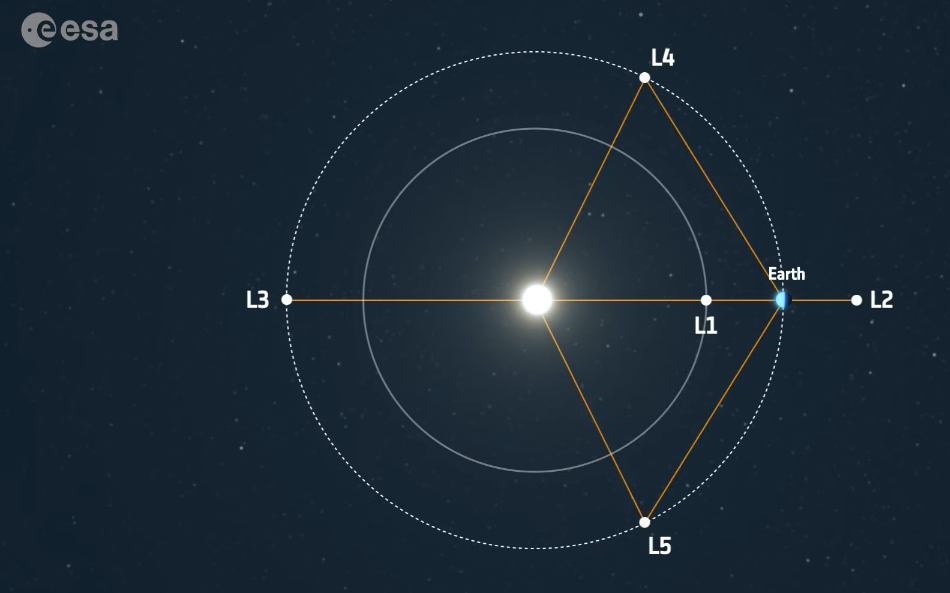
Lagrange found the equilibrium solutions (the five Lagrangian points, see figure taken from the ESA website) for the system in the simplified yet highly interesting case where the third body has negligible mass compared to the other two (e.g., the Sun, a planet, and an asteroid or an artificial satellite). The first three points (L1, L2, L3) had already been found by Leonhard Euler (1707-1783), another huge mathematician of the 18th century, while Lagrange found the so-called ‘triangular’ points (L4, L5), because they form perfect equilateral triangles with the two main bodies.
For details about these points, please refer to the easy explanations on the
link  ESA (European Space Agency) website.

Obviously, Lagrange could never have known about the evidence supporting his conjecture (it was only in 1906 that astronomers confirmed his theory by discovering Trojan asteroids captured at points L4 and L5 of Jupiter’s orbit) or its current usefulness in positioning our space exploration vehicles.
Thanks to their ‘gravitational stability’, which saves positioning energy (and in the case of L2 also provides partial shielding from the Sun), it is conceivable that, in the future of space exploration, advanced bases for deep space exploration will be located at Lagrangian points.


The 5 Lagrangian points, from the link  ESA (European Space Agency) website; the orbits of points L1 and L2 are not to scale, the distance from Earth is about 1/100 of the radius of Earth’s orbit.

Lagrangian points

please, rate this post

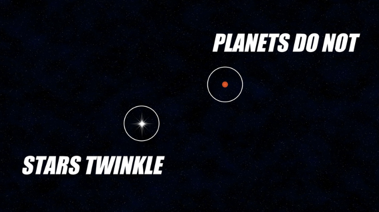
Why do stars twinkle at night and planets do not?

planets do not twinkle
This fact, known for millennia, allows even the layman to immediately distinguish in the night sky one of the planets of the Solar System (Venus, Mars, Jupiter, Saturn) from the stars with the naked eye.
These light sources, observed from the Earth’s surface, exhibit two main characteristic behaviors due to the same cause, atmospheric turbulence:
– slight oscillations in position (appreciable with good binoculars or a small telescope)
– intensity twinkling (typically only stars).
Other effects, especially when the source is close to the horizon, are: chromatic twinkling (color changes), atmospheric extinction (decrease in brightness), reddening, and twinkling of the planets.
Atmospheric turbulence at low altitudes (the first tens or hundreds of meters) is responsible for positional oscillations, together with turbulence at medium altitudes (6-8 km) where air cells of different temperatures and densities mix, while turbulence near the tropopause (8-12 km) associated with jet streams is responsible for scintillation.

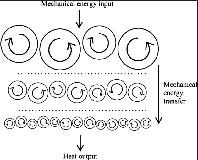
It is the optical dimensions of the sources that make the difference in the scintillation, based on their interaction with turbulence cells, which also vary in size. Jet streams determine large cells, ranging from tens to hundreds of meters, but turbulence follows Kolmogorov’s cascade model (see Figure 1), dissipating the initial kinetic energy into increasingly smaller vortices, down to the order of centimeters or millimeters, eventually dissipating into heat. It is precisely these microcells that deflect the point-like light from stellar sources, but they have a mediated effect in the case of optically larger sources such as planets, which involve multiple cells. The final effect is the stabilization of the source’s light, which therefore appears non-twinkling.


Figure 1 – An illustrative sketch of turbulence transformation according to Kolmogorov’s cascade model

turbolence

please, rate this post

The equal sign “=”

Some considerations for true beginners.

The equal sign “=” is a mathematical symbol (coined by Welsh mathematician Robert Recorde in 1557) of two parallel horizontal lines used to show that two expressions have the same value or are identical.
It is taught very early on in elementary school, but I don’t think the power of its deep meaning is explained well. At least, that’s what we can see from the difficulties experienced by slightly older students.

Equal means exactly equal. What is on the left of the “=” sign has the same value as what is on the right. So if there is a symbol on the left and a number on the right, in that context that symbol is worth exactly the amount indicated. And if two symbols are equal, they can be used interchangeably. Trivial, but a source of great doubt for those who have not fully grasped the basic concept.

From a formal point of view, the equal sign satisfies the following conditions:
– Reflexive Property: any value is equal to itself,  a = a
– Symmetric property: if  a = b  then  b = a  (the order of the expressions can be swapped without changing the truth)
– Transitive Property: if  a = b  and  b = c  then  a = c

– Substitution Property: informally, this just means that if  a = b , then  a  can replace  b  in any mathematical expression or formula without changing its meaning; formally, for every  a  and  b , and any formula  ϕ(x)  with a free variable  x , if  a = b , then  ϕ(a)  implies  ϕ(b) ; we can call this a function application.

Even without going into further detail, these simple properties allow us, for example, to solve first-degree equations directly. They allow us to invert formulas simply by adding or multiplying the same quantity on both sides of the equation. OK, taking care not to divide by zero.
If the unknown quantities (the so-called variables) are of a higher degree, things get more complicated, but the effectiveness of “=” remains the same.
A powerful little trick based on this is to use new variables to replace more complicated expressions or those with higher powers.

please, rate this post

References for laymen: an experiment to verify the law of falling bodies

The first observational measurements on the law of falling bodies were made by Galileo Galilei (1564-1642).
The famous law, considering the distance d traveled during the fall, is:
[1]    d = g t² / 2
where  g  is a constant representing the local gravitational acceleration (on Earth a mean value is  g = 9.8 m/s² ), and  t  is the time elapsed. In more easily observable terms, the fall time can be measured reversing the relationship  [1] :
[2]    t = √(2d/g)  .
Galileo predicted (inspired by what Domingo de Soto had already conceived in 1551) that all bodies follow this law regardless of their mass, studying rolling balls (rather than dropping them from the famous Tower of Pisa). However, everyday experience tells us that light bodies fall more slowly: this is simply due to the friction of the fluid in which they are immersed (e.g., air).

A rather expensive experiment was reported to have been carried out on the Moon, when a hammer and a feather were dropped and touched the ground at the same time (astronaut David Scott on August 2, 1971).
I propose the following more economical experiment: drop a coin that is not too small, for example a 2 euro coin, flat on its face, placing a small piece of paper, e.g. 5 mm in diameter, on top of it. A good height would be half a meter. You can observe that the piece of paper reaches the ground at the same time as the coin, which prevents the air from slowing it down.
You could also place the piece of paper in a transparent container that you then drop, but this would make it less clear to observe.

As a side note, it can be observed that a body in free fall accelerates until this acceleration equals the acceleration of gravity, due to the mass of the body (tipically the Earth) on which it is falling (possibly slowed down by air resistance, known as drag force). Once this is reached, the speed of fall, known as terminal velocity, remains constant. On contrary, a body falling in a vacuum never reaches terminal velocity because there is no drag force; it accelerates indefinitely as long as it is falling.

please, rate this post

References for laymen: how to use the sky to find your orientation

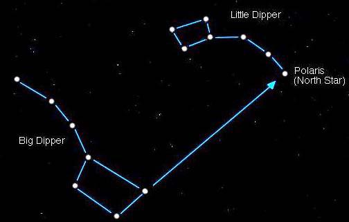
At night, everyone knows that North is roughly indicated by the North Star, which is easy to locate using the well-known asterism of the Big Dipper (and/or the slightly less prominent Little Dipper), see Figure 1.


Figure 1


During the day, however, the easiest direction to identify is South, which is accurately indicated by the Sun at its culminate point at noon every day of the year. Without having to wait for the culmination, knowing the time, you can estimate the direction of South by adding to the direction of the Sun at that moment (in the northern hemisphere, to the right in the morning and to the left in the afternoon) the angle missing to reach noon, considering 15° for each hour to midday (a full rotation of the Earth of 360° divided by 24 hours = 15°).
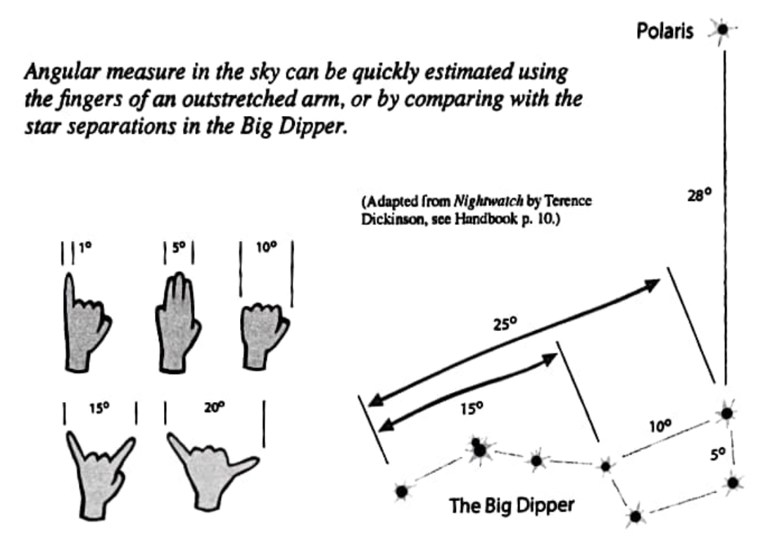
See Figure 2 for some practical references for estimating angles in the sky.

The height in degrees of the Sun above the horizon at its culmination point has been used for thousands of years to determine the observer’s latitude. Eratosthenes of Cyrene (276-194) used it to calculate the circumference of the Earth in a way that was effective for the knowledge of the time.

And again, thanks to knowing the exact ‘universal’ time, you can determine the longitude by converting the hours/minutes difference between the local culmination time of the Sun and the culmination time at longitude zero, taken as a reference, at the Greenwich meridian, into degrees. Obviously, east of this meridian, the culmination will be earlier, while west of it, it will be later.
This principle has also been known for centuries. However, it was possible to exploit it only when clocks of sufficient precision and reliability were built (at the beginning of the 18th century, mainly thanks to John Harrison, see for example Longitude, Dava Sobel, Walker Publishing Company, 1995).

To obtain accurate measurements, precision instruments (like a sextant) are obviously required (apart from the GPS available in every cell phone today!), but for a rough estimate, the above is sufficient.


Figure 2 – Easy reference for measuring angles in the sky (image credit: Nightwatch, Terence Dickinson)

angles in the sky

please, rate this post